Dealing With Missing Values, Part 3.

More Advanced Methods

This is the third and last post on the topic of dealing with missing values in Data Science and Machine Learning. You can read the first part here, and the second part here. As I noted in my first post in this series, this turned out to be a much bigger topic than I had though when I first wrote about it years ago, and what I intended to be a quick short post ended up needing to be split into three parts. Even so, we have only scratched the surface of this big area, and you are urged to look up many other wonderful sources online.

So here are three more ways of dealing with missing values.

Probabilistic & Statistical Approaches (Bayesian/EM-style)

When handling missing data, probabilistic and statistical approaches are valuable because they explicitly model missingness under a rigorous framework. Methods like Expectation-Maximization (EM) iteratively estimate missing values alongside the parameters of the underlying statistical model, offering a structured and statistically sound solution. One effective implementation in Python involves scikit-learn's IterativeImputer coupled with a BayesianRidgeestimator. This combination iteratively imputes missing values by treating them as random variables, leveraging Bayesian inference to incorporate uncertainty and manage complex multivariate relationships. Bayesian methods specifically allow for incorporating prior information, which can enhance robustness, particularly in scenarios with limited data or small sample sizes. This can be especially beneficial when dealing with sensitive or critical datasets in fields such as healthcare, finance, or scientific research, where the cost of incorrect imputations can be high.

For instance, in Python, you might write:

Interpolation (Time-Series & Ordered Data)

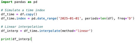
Another effective method, particularly suitable for sequential or ordered data such as time-series, is interpolation. Interpolation techniques fill in missing data by estimating values based on surrounding known data points, thus preserving continuity and inherent sequential patterns. Linear interpolation, which connects missing points using straight lines, is common due to its simplicity and effectiveness. However, more sophisticated methods like spline or polynomial interpolation can be utilized if smoother transitions are desired, although these might introduce artifacts, especially in noisy datasets. Moreover, interpolation techniques are highly context-sensitive; they assume that sequential order or time intervals between observations accurately reflect underlying trends or patterns. Therefore, careful assessment of data continuity and frequency is essential before selecting an interpolation method.

A straightforward interpolation example in Python might look like:

Robust Model Design (Tree-Based & Native Missing-Value Handling)

Alternatively, some algorithms natively handle missing data, particularly tree-based models such as scikit-learn’s HistGradientBoostingClassifier, XGBoost, LightGBM, and CatBoost. These models inherently manage missing values during training, eliminating the need for a separate imputation step and often resulting in excellent predictive performance. They manage missing data by internally identifying optimal splits, taking missing values into account directly during model training. Although these methods simplify preprocessing, they limit your model selection flexibility by tying you to specific algorithms. Additionally, models with built-in handling of missing values may also yield more interpretable outcomes since they clearly illustrate the role of missingness within the predictive structure.

Here's a brief example:

How to Choose the Right Method

Choosing the right method for dealing with missing values involves thoughtful consideration of several factors. Understanding the underlying mechanism causing missingness is critical. Data that are Missing Completely at Random (MCAR) are typically easier to manage with simpler methods like mean or median imputation. Missing at Random (MAR) data may require more sophisticated techniques such as multivariate imputations (e.g., MICE), as these methods better capture complex relationships among variables. Data Missing Not at Random (MNAR), meanwhile, usually necessitate domain-specific insights or specialized statistical approaches, possibly including sensitivity analyses or explicitly modeling the missingness mechanism itself.

It is essential to evaluate how each method impacts your dataset's integrity and potential biases. While deletion methods are straightforward and computationally simple, they might substantially reduce the dataset's size and introduce bias, especially if data are not missing completely at random. Simple methods, such as mean or median imputation, can be useful initial steps to benchmark results and provide baseline performance. Progressing toward more sophisticated approaches like KNN or MICE is advisable as the complexity of the data and analysis requirements grow. These advanced methods, while computationally more intensive, typically yield higher quality imputations by capturing interdependencies among features.

Domain knowledge remains invaluable throughout this process. Incorporating expert insights can guide sensible thresholds or plausible imputations, significantly enhancing the validity and reliability of your analyses. Practical considerations, like data collection methods, measurement errors, and domain-specific data constraints, should always inform your choice of imputation strategy. Finally, remember that methods can be combined creatively. For instance, interpolating sequential data before using a robust tree-based model, or employing missingness indicators alongside probabilistic methods, can offer practical and effective solutions.

By carefully applying these strategies, you can effectively manage missing values, leading to more accurate, reliable, and insightful outcomes in your data science and machine learning projects.