XGBoost is All You Need - Part 6

Nontrivial use case 2: use of Shapely values for feature selection and feature engineering

This is the sixth installment in my series of posts on XGBoost, and the second on practical applications, based on my 2024 GTC presentation. Previous posts can be found at the following links: Part 1, Part 2, Part 3, Part 4, Part 5.

Shapley Values - The power of interpretability

Shapley values are a unique, game-theoretic approach to attributing feature importance in machine learning models. Originating from cooperative game theory, Shapley values were originally designed to fairly distribute a coalition’s payoff among players based on their contributions​. In the ML context, each feature value is treated as a “player” in a game where the model’s prediction is the total payout to be distributed​. This provides a theoretically sound framework for feature attribution: Shapley values are the only solution that satisfies certain fairness properties (efficiency, symmetry, dummy, additivity) that ensure each feature gets credit proportional to its true contribution​. In contrast, simpler heuristics like the built-in feature importance of a tree model (e.g. Gini importance or split counts in random forests) lack such rigorous guarantees and can be biased by factors like feature scale or redundancy. By fairly allocating credit to features, Shapley values offer a more principled measure of importance for tasks like feature selection – helping identify which features genuinely drive the model’s predictions as opposed to those that appear important due to quirks of the training process.

Shapley values provide local, instance-level explanations. Unlike global feature importance methods that yield a single importance score per feature (averaged over all data), Shapley values break down each individual prediction into contributions from each feature. In other words, for every data point, we get a personalized attribution of how each feature influenced that particular prediction. This local explanation property is extremely powerful: it means we can explain why the model made a specific prediction by looking at that data point’s Shapley values (e.g. “Feature A contributed +0.5 to the prediction, Feature B contributed -0.2,” etc.). SHAP (SHapley Additive exPlanations) is a popular framework that leverages Shapley values for per-instance explainability​. For example, suppose a tree model ranks “Income” as the most important feature overall for loan approval (global importance). Global methods tell us Income matters on average, but they won’t explain why two particular applicants with similar income got different outcomes. Shapley values, however, can reveal that for one applicant, Income had a high positive contribution, while for another applicant Income had a smaller effect and another feature (say, Debt) drove the prediction. This per-instance granularity contrasts with global importance metrics like permutation importance, which lack context for individual predictions.

The downside is that exact Shapley value computation is notoriously expensive — the complexity grows exponentially with the number of features. Computing a feature’s Shapley value involves considering all possible subsets of features and measuring the feature’s contribution in each context. Formally, for N features, there are 2^N possible subsets (coalitions) of features, and evaluating all of them for every feature quickly becomes intractable as N grows. In fact, a straightforward calculation requires on the order of N! (factorial) evaluations to get exact Shapley values, which is computationally prohibitive except for very small feature sets​. This exponential explosion means that if you have, say, 20 features, the number of coalitions to examine is over 1 million; with 30 features it’s over a billion. The factorial growth of subsets makes exact Shapley calculations infeasible for high-dimensional datasets or complex models​. In practical terms, evaluating every combination of features would require an astronomical number of model runs, so exact Shapley values are rarely computed for real-world ML problems. Data scientists must therefore be mindful of this trade-off: while Shapley values are theoretically appealing for feature importance, naively computing them doesn’t scale. This limitation has driven the development of clever approximation methods to make Shapley-based explanations usable in practice.

Most Shapley value implementations rely on approximation techniques or model-specific assumptions to sidestep this combinatorial explosion. To make Shapley values feasible, researchers have developed algorithms that approximate the exact values with far fewer evaluations. A common strategy is Monte Carlo sampling: rather than enumerating all 2^N subsets, one can sample a large number of random feature orderings or subsets and estimate each feature’s average marginal contribution from those samples​. . The SHAP library popularized this approach, providing a unified framework for approximating Shapley values for any model by treating the explanation as a weighted linear regression problem (KernelSHAP). For tree-based models, there is an even more efficient method known as TreeSHAP, which exploits the tree’s structure to compute Shapley values in polynomial time instead of exponential​. TreeSHAP uses dynamic programming on decision paths to exactly compute Shapley contributions for tree ensemble models much faster than brute-force. In practice, tools like the SHAP Python package use these techniques under the hood: for arbitrary models it uses sampling-based approximations, and for decision tree models (e.g. Random Forests, XGBoost) it uses the TreeSHAP algorithm for speed​. The key point is that virtually all Shapley value software avoids the full exponential cost by leveraging approximations or optimizations. While these methods may introduce a bit of approximation error, they make it practical to get Shapley-based feature importances on datasets with dozens or even hundreds of features. Thus, data scientists can reap the benefits of Shapley values’ fairness and local accuracy without waiting millennia for computations to finish.

Because calculating Shapley values (or their approximations) involves repeated model evaluations for many feature combinations or permutations, the problem is embarrassingly parallel. This means it can benefit hugely from parallel hardware like GPUs. GPUs can execute thousands of operations simultaneously, making them well-suited to speeding up the large number of independent calculations required for Shapley estimates. In recent years, GPU-accelerated implementations of SHAP and TreeSHAP have shown order-of-magnitude speedups. For example, one study reported achieving up to 19× faster computation of standard Shapley values and up to 340× faster computation of Shapley interaction values by offloading the work to an NVIDIA V100 GPU, compared to a multi-core CPU baseline​. Libraries such as GPU TreeShap (integrated in frameworks like XGBoost) allow Shapley values for tree models to be calculated on GPUs, often turning hours of computation into minutes. The SHAP Python library can also utilize GPU backend (via CuPy or GPU-enabled tree libraries) to accelerate KernelSHAP sampling and TreeSHAP calculations. For data scientists, this means that computing Shapley explanations on large datasets or complex models is no longer prohibitive – with the right hardware and libraries, you can get near real-time explanations.

Shapley Interaction values – an extension of Shapley values – are useful for uncovering feature interactions and informing feature engineering. So far we’ve discussed allocating importance to individual features, but Shapley analysis can go a step further and quantify the contribution of feature combinations. Shapley interaction values allocate credit among pairs of features (and by extension, can be generalized to higher-order groups)​. In essence, they decompose the prediction not just into single-feature effects but into pairwise interaction effects as well. For two features i and j, the Shapley interaction value attempts to measure how much those two features together contribute to the prediction beyond the sum of their individual contributions. Concretely, SHAP interaction values produce a matrix of attributions: the diagonal elements are the usual Shapley values for each feature (solo effect), and each off-diagonal element is the attribution for the interaction between feature i and feature j. This tells us whether the model has learned any synergy or redundancy between features. For example, if features X1 and X2 only matter when combined (perhaps they represent coordinates that together pinpoint a location), Shapley interaction values for the pair (X1,X2) will be high, indicating a strong synergistic interaction. Conversely, if two features provide overlapping information (one might make the other redundant), the interaction value for that pair will be near zero or even negative, indicating that knowing both doesn’t add much beyond one alone. Identifying such relationships is extremely valuable for feature engineering: redundant features can potentially be pruned to simplify the model without sacrificing performance, while synergistic features might inspire creation of a new combined feature or at least inform us to keep both features together​. Shapley interaction values thus enable data scientists to dissect not just individual feature effects but also the pairwise dependencies learned by the model. This insight can guide feature selection (e.g. avoid dropping a feature that only has importance when partnered with another) and feature creation (e.g. adding interaction terms or aggregated features). Overall, by extending the fair credit allocation principle to feature pairs, Shapley interaction values provide a systematic way to quantify feature interactions, shining a light on complex relationships that simpler importance metrics would miss.

Shapley values in XGBoost

Starting with XGBoost v1.3 (released in late 2020), the library introduced GPU acceleration for Shapley value computations​. One convenient feature of XGBoost is that its standard Python API can compute Shapley values directly. By simply calling the model’s predict method with pred_contribs=True, XGBoost will return the contribution of each feature to the prediction (the Shapley values) without any external libraries​. This built-in functionality means you don’t need third-party packages to derive feature importance via Shapley values – the logic is integrated and optimized within XGBoost itself. In practice, this tight integration makes computing feature attributions more efficient. For example, one user reported that using the standalone SHAP library took days on a subsample of a dataset, whereas XGBoost’s native method produced the same Shapley values in just minutes​. Eliminating the extra overhead of external explainers thus streamlines the workflow and speeds up the calculations.

In addition to individual feature contributions, XGBoost’s API also supports computing Shapley interaction values directly. By setting pred_interactions=True in the predict call, you can obtain second-order Shapley values that attribute contributions to pairs of features​. This allows data scientists to analyze feature interactions (how two features jointly influence a prediction) without needing any external implementation. The ability to get interaction effects natively is particularly useful for understanding dependencies in tree-based models – for instance, it can reveal whether two features together have a synergistic or compensatory effect on the model’s output. All of this is done within XGBoost’s own engine, again avoiding the need to hand data off to another library for these deeper insights.

GPU acceleration has been a game-changer for applying Shapley values to larger datasets. Prior to GPU support, analysts often had to sample down their data or limit Shapley calculations to a handful of instances due to the heavy runtime. Now, with orders-of-magnitude faster computation, it’s feasible to explain predictions on extensive datasets or very complex models. The ability to harness a GPU (or multiple GPUs) effectively removes the previous scalability barrier​. Data scientists can obtain comprehensive feature attribution on datasets that were once too large to handle, without waiting days for results. In short, the introduction of GPU power has made Shapley-based interpretation practical for big data scenarios that were previously off-limits.

In practice, the speedups from GPU acceleration are often on the order of hundreds-fold, and in some cases even 1000X or more faster compared to CPU-only methods. The exact gain depends on factors like the size of the dataset, number of trees, and hardware specifics, but it is consistently very large. These massive speed improvements mean that tasks which previously might have timed out or taken unbearably long can now be completed quickly. Even with a modest GPU, you can expect a substantial reduction in computation time for Shapley value analysis, often turning a formerly overnight job into a matter of seconds or minutes.

Because of this dramatic acceleration, XGBoost users can incorporate Shapley value explanations into real-time or iterative workflows. For instance, you could generate explanation values for new predictions on the fly in a production setting, or interactively explore feature effects in a Jupyter notebook without long delays. Multi-GPU setups push this even further – one benchmark achieved about 1.2 million rows per second throughput when computing SHAP values using eight GPUs in parallel​. This level of performance was unimaginable with earlier CPU-only methods. It enables high-volume inference monitoring or dynamic dashboards that explain model decisions almost instantly.

SHAP package

The SHAP library provides a highly intuitive Python interface for computing Shapley values, making model interpretation accessible to data scientists. Its API is well-documented with plenty of examples, so you can quickly learn how to explain your models’ predictions. SHAP integrates smoothly with popular machine learning frameworks and supports a wide range of model types. In practice, you can plug in models from scikit-learn, XGBoost, LightGBM, CatBoost, or even deep learning frameworks and obtain Shapley value explanations with minimal code. Many common model objects are directly supported – for example, tree models from XGBoost, LightGBM, CatBoost, PySpark, and scikit-learn work out-of-the-box with SHAP’s explainer classes​. This broad compatibility and user-friendly design have made SHAP a go-to tool for interpretable machine learning.

SHAP doesn’t just stop at computing values – it also includes excellent built-in visualization tools to help make sense of the results. These plots are designed to be interactive in Jupyter notebooks, leveraging JavaScript behind the scenes for rich displays​ (the library provides an initjs()function to load the necessary JS components when needed). Two key visualization types are the summary plot and the force plot.

• Summary Plot: This chart provides an overview of feature importance across the entire dataset. It typically appears as a beeswarm or layered scatter plot where each point is a Shapley value for a feature in one sample. In a single view, you see which features are most influential (ranked by overall impact on the model output) and how their values affect the prediction (color indicating feature value). In essence, the summary plot gives an overview of the most important features across the entire dataset​.

• Force Plot: For understanding individual predictions, SHAP offers the force plot, which visualizes how each feature pushes an individual prediction higher or lower relative to a baseline. A force plot is a dynamic, bar-like visualization (often shown as an interactive red and blue force diagram in Jupyter) for a single observation. It displays the contribution of each feature value as a force that either increases the prediction (positive Shapley value pushing to the right) or decreases it (negative value pushing to the left) from the model’s base value. Essentially, the force plot “shows how the features of a data point contribute to the model’s prediction”​.

Shapely values with Porto Seguro and XGBoost

We are now going to illustrate the above features, easy fast Shapely values calculations with XGBoost and easy visualization with the SHAP package, using the Porto Seguro dataset that we had mentioned in the previous post. We assume that we have already found the optimal hyperparameters for the dataset, and have trained a model with them. We will now calculate the Shapely values and the Shapely interaction values for the validation dataset, and we’ll use an H100 GPU to do so. Thanks to its speed and relatively large vRAM size (80 GB), both of these calculations can be done pretty fast and the results fit easily in memory, something that is not always the case, especially for the Shapley interaction values.

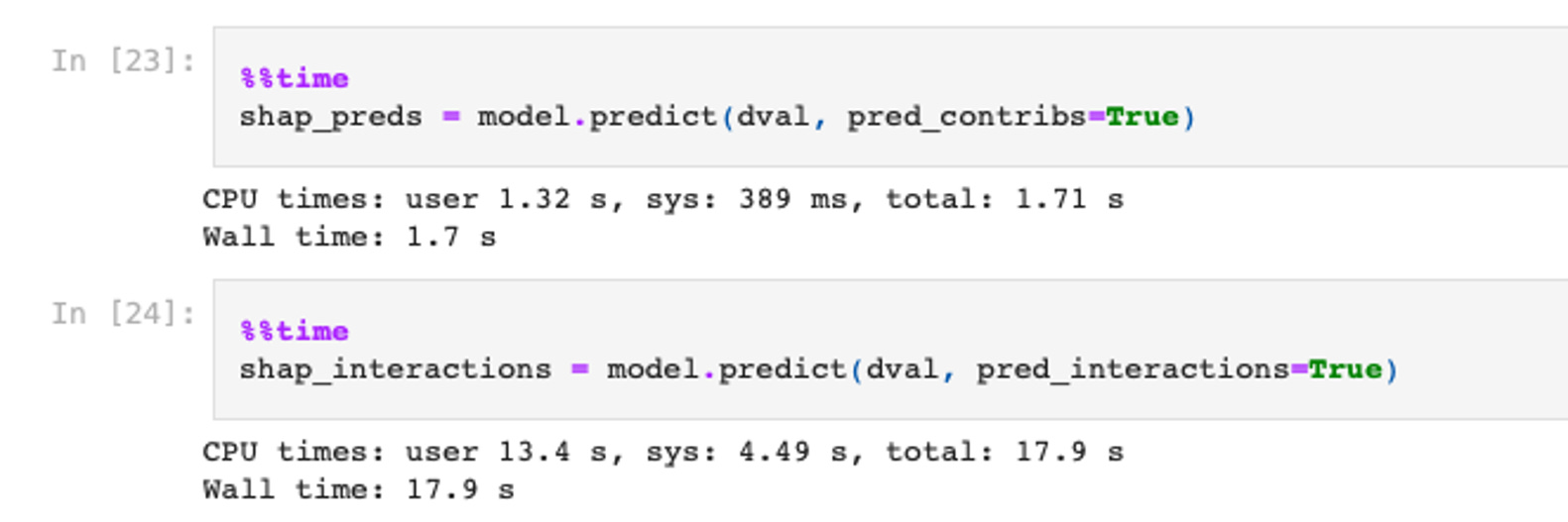
Once we obtain these values, we use SHAP’s excellent visualization tools to display them, both average absolute value for each feature, as well as their overall per-datapoint distributions. The average absolute value of each feature looks like the following:

This plot tells us which features are the most important. Unfortunately, in this dataset all features are anonymized, so we cannot really try to get any deeper insights about them, or use any kind of domain-specific knowledge to engineer those features further in order to extract more predictive information out of them. However, with non anonymized plots such insights could prove to be invaluable.

Next, let’s take a look at the feature importance distributions:

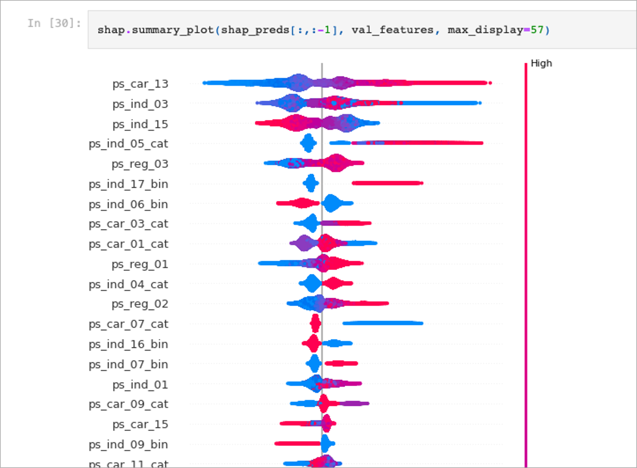
This SHAP summary plot shows each feature’s influence on the model’s output across all validation samples. The features are listed in descending order of overall importance (i.e., how much each feature contributes, on average, to the model’s predictions). For each feature, the horizontal spread of colored points captures the range of possible Shapley values, which can be interpreted as how strongly (and in which direction) that feature affects individual predictions.

A positive SHAP value (points to the right of the vertical line) indicates that the feature value pushes the model output higher, while a negative value (points to the left) means it pushes the output lower. The color scale (blue to pink/red) shows the feature’s actual value: blue typically represents lower feature values, and pink/red represents higher values. Taken together, you can see patterns such as “higher feature values lead to higher (or lower) predictions” if most of the pink points are clustered on one side. For instance, a feature where pink points mostly lie on the right side of the vertical line suggests that high values of that feature increase the predicted outcome. Conversely, if blue points concentrate on the right side, then lower values of that feature tend to raise the model’s prediction.

Looking at the topmost features, you can see they have wide spreads of SHAP values, indicating they strongly influence the model’s output. Lower-ranked features have a narrower range, so they contribute less on average. Overall, this chart helps identify which features matter most (the ones at the top) and how different feature values shift each prediction up or down.

Next, let’s take a look to see if there are any features that don’t make any contribution to the overall absolute Shapley values. These features should almost always be dropped. The only exception is if their interaction with other features is nonzero, but even there, unless those interactions are pretty significant, it’s most likely that it would be fine to just drop them anyways.

We’ve identified six “faulty” features that need to be dropped. After retraining the model on the dataset with those features removed, the score improves slightly from 0.2851 to 0.2859. This is to be expected, and in fact probably underestimates the impact of those “faulty” features on the model. To get a more accurate assessment, we should re-do the hyperparameter optimization. However, in most practical situations this extra step might be an overkill.

Shapely interactions and Feature Engineering

The above example is an instance of feature selection, where we decide on which features to keep and which ones to discard based on how much they contribute to the overall score in terms of their absolute Shapley values. However, without actually knowing the meaning of the features, it’s not really feasible to use feature importance as the basis for feature engineering - a process of constructing new features based on transformation of individual features or the combinations of them. This is where Shapley interaction values can come in handy. We can relatively easily build new features based on our knowledge of which feature interactions are the strongest. Let’s take a look and see how to do it.

We write a new function, plot_top_k_interactions, which computes mean absolute SHAP interaction contributions for each pair of features and then plots the strongest ones as a bar chart. It first slices out the bias term from shap_interactions and takes the average across samples, resulting in a two-dimensional matrix of mean interaction strengths. It iterates through that matrix to build a list of (feature_pair, interaction_strength) tuples, skipping duplicates by only taking lower-triangle indices (j < i) and multiplying each average by 2 to account for symmetric entries. The list is then sorted in descending order by interaction strength. Finally, it extracts the top k pairs, plots them using a basic bar chart (rotating the x-axis labels to avoid overlap), and returns the full list of sorted interactions. This allows us to quickly see which feature interactions have the largest influence on model predictions, aiding in feature engineering and interpretability.

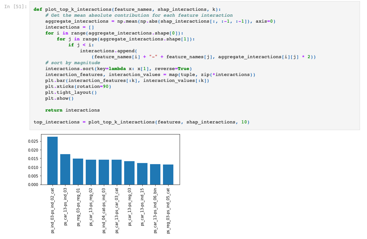
Next, we take the top two feature interactions, and create two more simple features that are just products of the individual features:

And then, as in the previous section, we retrain the XGBoost model, with the original hyperparameters, and our validation score improves further, from 0.2859 to 0.2871. The improvement seems more significant than the improvement that we got from feature selection. This might be just a fluke, but in my experience feature engineering is generally a far more productive step than feature selection. However, a simple multiplication may not always work. Oftentimes it is necessary to use a different way of combining the features, especially when at least one of the two features is categorical.